SPARQL Debugger and Profiler View

SPARQL queries may get complex and often contain a series of operators such as triple matches, filter clauses, optional statements and unions. In many cases, building correct and efficient queries using those elements requires multiple attempts. This is often because it is difficult to see what the SPARQL engine is doing under the hood.

The Debugger View has been designed to help query designers by providing an interactive view into a query at execution time. The Debugger can be used to:

• Display the internal data structure (algebra) that the SPARQL engine is using to execute the query
• To walk through the execution of the query
• To display intermediate variable bindings
• To execute a query until it reaches a certain break point
• To collect statistics about the number of query steps involved in every operator

This is a sophisticated feature that can be extremely powerful, but it also requires a decent understanding of how SPARQL works. People with some programming background may find the debugger more useful than beginners.

Background

Let's start with some background on how SPARQL works. The key feature of SPARQL is the WHERE clause, which contains conditions that return variable bindings based on the query graph. Depending on the type of query, these variable bindings are then returned in the SELECT clause, or used to CONSTRUCT new triples. In order to understand the characteristics of a query, we therefore need to focus on the WHERE clause, and modifiers such as ORDER BY.

When a query is processed, the SPARQL engine will first create an internal data structure, called Algebra. The query is executing this data structure, while the textual representation with keywords such as SELECT and WHERE only serves as the user interface and query exchange language. It is important to understand that different query syntaxes may be converted into the same algebra data structure, and that the same query syntax may be rendered into different algebras depending on the choices of the SPARQL engine. In particular, the engine may decide to optimize certain patterns. Seeing the internal data structure will often lead to surprising results.

For example, the query

SELECT ?subject ?object
WHERE {
    ?subject rdfs:subClassOf ?object .
    ?subject rdfs:label ?label .
    FILTER (fn:starts-with(?label, "C")) .
}

is converted into a SPARQL Algebra data structure that can be rendered into textual form as follows:

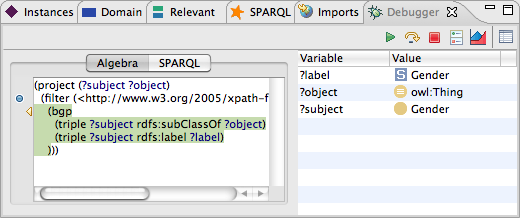
(project (?subject ?object)
 (filter (fn:starts-with ?label "C")
   (bgp
     (triple ?subject rdfs:subClassOf ?object)
     (triple ?subject rdfs:label ?label)
   )))

In this notation, you can see that the SPARQL engine is working with a nested tree structure of operators such as project, filter and bgp. These operators typically have attributes or child elements, for example bgp (Basic Graph Pattern) contains a list of triple patterns to evaluate. Note that it is up to the SPARQL engine to optimize those operators so that they lead to fewer database requests. In particular, multiple triple matches may be combined to a single operation to benefit from server-side joins.

The Algebra operators form a tree structure, in which each node returns an iterator of variable bindings. For example, the basic graph pattern above may return the binding ?label="Matriarch"^^xsd:string, ?object=Person, ?subject=Matriarch. These bindings are served up to the next operator in the processing pipeline. For example, the filter operator will evaluate whether the ?label starts with "C" and then pass the same bindings to its parent operation, the project step. Thus, each operator receives a stream of input bindings and may create new bindings for its parent. The final results of the query are the output bindings of the root operator (here, project).

The algorithm of the SPARQL engine (at least the Jena ARQ engine used by Composer) follows the evaluation model above, and builds a nested hierarchy of iterators. Each of those iterators has two main functions:

1. hasNext to check whether there is any additional result binding available
2. next to return the next binding and move to the next step

The SPARQL Debugger allows users to trace the evaluation of the SPARQL engine to see when hasNext and next are invoked, and whether they return new variable bindings. When you step through the query manually, the user interface will display arrows in different colors to illustrate the current position, and display variable bindings in a table.

Getting Started with the Debugger View

TopBraid Composer's SPARQL Debugger is accessible from multiple places:

• In the SPARQL View, use the Debug query button to open the currently edited query in the Debugger view.
• In the context menu of spin:rule property values on the form, use Debug SPIN query to debug the SPIN rule. Note that this may add a clause ?this rdf:type [Class] to the query, just like the SPIN engine would do.

As shown above, the Debugger is split into multiple areas. The main area on the left displays the query. Two different renderings are available:

• Algebra displays the internal Jena ARQ data structure
• SPARQL displays the same query in pseudo-SPARQL, which is derived from the Algebra (reverse engineered if you want) and therefore may look different from the original SPARQL syntax.

You can switch between those two renderings at any time and will get the same features. Depending on your experience, the SPARQL view might be easier to get started, but the Algebra view is much more informative as it provides the real underlying data structure.

Both textual views have a control bar on their left border. This bar displays the current step position with an arrow, and also displays any break points. Double-click on the bar to set or remove break points.

On the right hand side, a table displays current variable bindings. These are only filled if the current execution step is "green", i.e. is returning the next operation with some values.

The tool bar contains buttons to control the behavior of the SPARQL view. The following buttons are available:

• continues the execution of the query until the next break point.
• continues the execution of the query to the next step. The types of steps are described below.
• activates or de-activates profiling. When activated, the engine will record the triple matches (findSPO) queries done against the triple source, and display the resulting statistics behind each operation.
• switches between vertical and horizontal layout. Horizontal layout is better suitable for "wide" queries, vertical layout for lots of variable bindings.
• opens up the SPARQL Preferences page, which may impact how the SPARQL engine optimizes the query algebra. Changes will have effect after restarting the query.

Stepping through a query

When started, the query cursor will be (somewhere) at the beginning of the query data structure. Then, the following steps can be made to evaluate the query. These icons show up on the left control bar of the query views and point at the current position in the query.

• hasNext() is entered.
• hasNext() is exited with false.
• hasNext() is exited with true.
• next() is entered.
• next() is exited (always with a binding).

Using break points

Stepping through these phases manually may be slow and is very low-level. It is often more interesting to intercept the execution only at certain operations or positions. A break point is a marker that tell the debugger to stop at certain operations. Break points can be set using a double-click on the control bar to the left of the query view, or by double-clicking on an operation itself, inside the text view. There are two kinds of break points:

• stops whenever the operation is "touched", using either hasNext() or next() steps.
• stops only if a new binding for the operation has been found.

Substitutions

The SPARQL query engine may do substitutions of certain sub-operations at execution time. For example, if an OPTIONAL block is executed and refers to some variables that are bound in an operation before it, then the engine may substitute those variables to feed the OPTIONAL block with the right input.

If such a substitution happens while you are stepping through a query, the textual display will print the substitution below the original query. However, breakpoints, profiling statistics etc will be using the original query only.

Profiling

If profiling mode has been activated (and, if needed, the query restarted), then the query engine will operate on a modified triple store which, as a side effect of running queries, will also collect statistical information. In particular, this records which find(SPO) queries have been made, and how many triples have been iterated over. The accumulated numbers of those calls (find/triples) will be displayed for each operation in cyan color on the right edge of the text display. In the following example, there are two triple patterns that lead to low-level queries.

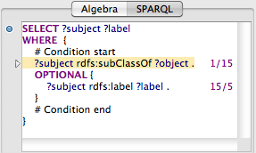
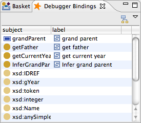
In the above screen shot, the upper triple match just leads to a single query (for all rdfs:subClassOf triples), and this query has (so far) returned 15 matches. The second (optional) triple match has been executed 15 times (for each of the former matches), but only five results were found so far. From these numbers you can see that the optional operation is far more "expensive" in terms of number of queries than the subClassOf query. The actual results of the query are shown in a separate window and updated whenever a new result comes in. You can see below that the five classes with labels are visible at the top, while the various XSD datatype resources do not declare an rdfs:label, leading to empty bindings from the OPTIONAL block.

Note that the results of the profiler need to be used with care, as the actual query performance strongly depends on the selected triple store. Many triple stores optimize the treatment of complex triple matches so that joins are made on the server. The profiler always counts individual triple matches, and therefore the actual number of requests may be much lower than the profiler displays it. Also note that the engine will run significantly slower if profiling is switched on.